Risk Curve and Capacity Model · BSC

The 17.98%→99.24% modeled decline, 120%→105% opening collateral ratio, and theoretical short-selling capacity by market cap.

Understand What the Model Does First

The risk model answers: At a given protocol market cap, how much cumulative net short selling is permitted? It does not predict prices or promise a maximum market decline.

The model first maps market cap to theoretical BNB reserves, then uses the specified price decline to calculate how much BNB may be removed. Executable capacity must also satisfy TWAP and spot constraints, lending inventory constraints, and Pair exact-output requirements.

Symbol	Meaning	Current BSC group value / unit
`M₀`	Ideal migration market-cap anchor	79.990424077961846080 BNB
`Mt`	Target market cap for risk / margin	70,000 BNB
`Q₀`	Ideal migration BNB reserve	15.998084815592369216 BNB
`T₀`	Migration Token reserve	2,000,000,000 Token
`S`	Curve supply	10,000,000,000 Token
`d`	Model price decline	bps, 1,798→9,924
`m`	Dynamic opening margin ratio	bps, 12,000→10,500
`C(M)`	Risk capacity at a given market cap	native18 BNB

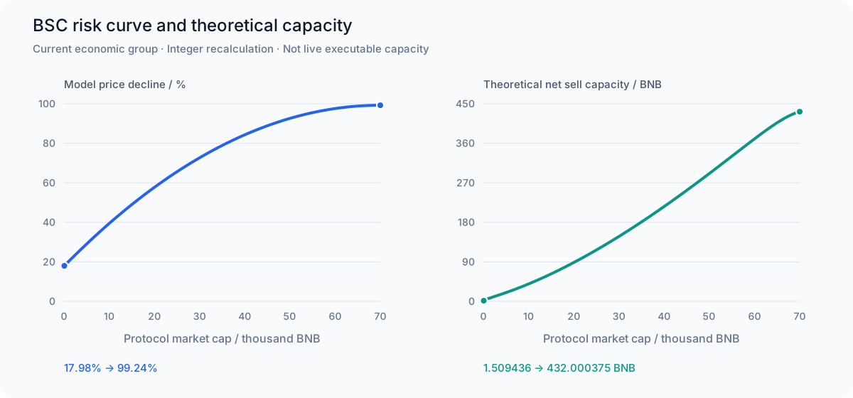
Current BSC risk decline and theoretical short-selling capacity

Chart capacities are recomputed with the current group’s integer implementation, before existing positions, TWAP constraints, or lending inventory constraints. Initial capacity is 1.509436282603634021 BNB and at the target market cap, 432.000375048343919998 BNB rather than rounded values shown in screenshots.

These values apply to the current economic group and need not be used by every subsequent group. Market capitalization continues to use the fixed curve supply of 10 billion Tokens and is not rescaled when the burn tax reduces the ERC-20 total supply.

1. Market-Cap Normalization

Risk capacity uses:

\bar M=\min\bigl(\max(M,M_0),M_t\bigr)

Continuous progress may be written as u = (M̄ − M₀) / (Mt − M₀). The actual implementation first quantizes this into integer bps:

u_{\mathrm{bps}}=\left\lfloor \frac{(\bar M-M_0)10{,}000}{M_t-M_0} \right\rfloor

The integer implementation therefore produces small steps rather than an infinitely precise smooth function.

When actual spot market cap falls below M₀, the model still calculates baseline capacity at M₀ ; it does not continue shrinking linearly to zero. Actual buyback prices, debt repayment, and liquidation still use the live Pair and are not protected by this market-cap floor.

2. Model Price Decline

Intuitive continuous formula:

d(u)=0.9924-(0.9924-0.1798)(1-u)^2

Corresponding integer implementation:

d_{\mathrm{bps}}=9{,}924- \left\lfloor \frac{8{,}126(10{,}000-u_{\mathrm{bps}})^2}{10{,}000^2} \right\rfloor

The starting point explicitly returns 1,798 bps; the endpoint returns 9,924 bps. This is a quadratic curve, not linear interpolation.

3. Dynamic Opening Margin Ratio

Intuitive continuous formula:

m(u)=1.05+0.15(1-u)^2

Integer implementation:

m_{\mathrm{bps}}=10{,}500+ \left\lfloor \frac{1{,}500(10{,}000-u_{\mathrm{bps}})^2}{10{,}000^2} \right\rfloor

The opening collateral baseline is notional times this ratio. See the detailed checks in Position Lifecycle.

Distinguish the two market-cap inputs: short capacity uses the market cap jointly constrained by the TWAP ceiling and spot; the dynamic opening ratio uses live market cap, floored at M₀. Do not directly substitute the capacity market cap into the margin curve.

4. Theoretical Reserves and Maximum Net Short-Sale Proceeds

Assuming the ideal reserve product is fixed at K₀ = Q₀T₀, the continuous model gives:

\widehat Q(M)=\sqrt{\frac{M Q_0 T_0}{S}}

\frac{P_{\mathrm{after}}}{P_{\mathrm{before}}} =\left(\frac{\widehat Q-C}{\widehat Q}\right)^2

Setting this ratio equal to 1 − d yields the intuitive capacity formula:

C(M)\approx\widehat Q(M)\left(1-\sqrt{1-d(M)}\right)

Integer Execution Order in the Contract

The following operations all use raw units, without substituting floating-point approximations:

z=\left\lfloor\frac{\bar M Q_0}{S}\right\rfloor, \qquad \widehat Q=\left\lfloor\sqrt{zT_0}\right\rfloor

R^2=\left\lfloor \frac{\widehat Q^2(10{,}000-d_{\mathrm{bps}})}{10{,}000} \right\rfloor

C(M)=\widehat Q-\left\lceil\sqrt{R^2}\right\rceil

Q̂ is a theoretical reserve, not the current Pair balance; the model's risk anchors are not rewritten when someone donates WBNB to the Pair.

5. Guarantees the Model Does Not Provide

Reaching a particular spot market cap does not immediately release all capacity associated with that level; TWAP may not yet confirm it.
Capacity is a cumulative net-sale limit, not collateral a user can withdraw or profit a user can earn.
If existing positions exceed contracted capacity, capacity for new positions becomes zero; liquidation eligibility is determined by position solvency.
The model does not cover changes in external liquidity, every price path, MEV, congestion, or execution slippage.